[ad_1]
An obscure economic indicator demands a reappraisal, both for its predictive value as well as its ironic origins in the old-style monetarism of Milton Friedman.
Of all the fads of the 1980s, the meticulous money-supply targeting recommended by monetarist economists packed more of a jolt than boom boxes, big hair, and “E.T. phone home” combined. The decade began just as the novel economics concept was working its way into the US Federal Reserve’s policy processes.
The Fed primarily targeted the M1 money supply, M2 on occasion, and also monitored M3 while experimenting with M1B and, later, MZM.
And alongside these official measures, monetarists concocted their own home-brewed variations and helped feed a national obsession with the money supply.
Policymakers left interest rates untethered so they could prioritize money, and rates soared and dipped even more wildly than they expected. This unprecedented interest rate volatility meant investors, borrowers, and bankers, especially, kept a sharp eye on developments, studying every wiggle in every M. To miss one could have been the difference between exploiting or succumbing to the volatility the Fed had unleashed.
And then, just as quickly as the frenzy blew in, it blew right back out. The Fed once again recalibrated its approach, first deemphasizing and then abandoning its money-growth targets.
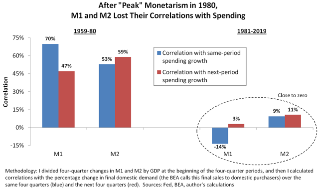
And with M1, M2, et al., showing little success as leading indicators, the monetarists exited the stage. Their heyday was over. William Poole summed up their miscalculation: “Those of us who have developed strong theories tried to fit the world into the theory rather than the other way around.”
Lesson learned. Rise and fall complete.
The flameout of the monetarists didn’t mean their insights were useless or irrelevant, however. On the contrary, the accomplishments of Milton Friedman and Anna Jacobson Schwartz, among others, were immense. Their economics gave the Fed the cover it needed to confront and defeat the devastating inflation of the 1970s and early 1980s.
The problem was in the aggregates the monetarists devised: They stopped working. M1 and M2 lost their correlations with spending.

Money and Banking: Two Descriptions
Why did these correlations evaporate? The answers lie in the poorly understood mechanics of our monetary system.
Consider two competing descriptions of money and banking:
| Description A | Description B | |
| Money Supply: | is controlled exogenously by the central bank. | is mostly determined endogenously by commercial banks and their customers. |
| Commercial Banks: | are mere intermediaries that receive deposits (money) and lend them out. | create new deposits in the process of making loans or buying securities. |
| Bank Loans: | come after deposits. | come before (create) deposits. |
Most people would agree with Description A and raise a suspicious eyebrow at Description B. In a common interpretation of the former, banks can only extend loans using the funds they have on hand. Another interpretation holds that Description A is accurate but Description B can still be true, in part, due to the money multiplier theory.
Description A is so popular because the standard textbooks teach it. We were all taught this way and whether we remember or not, commentators who were taught exactly as we were will repeat this doctrine ad nauseam.
But here’s the thing: Ample evidence shows Description B reflects reality better than Description A. Moreover, that evidence is more accessible today than ever before. The Bank of England sought to eliminate any confusion and explained why Description A is fallacious in “Money Creation in the Modern Economy” in 2014. And the BOE is hardly a voice in the wilderness. Among other banking authorities, the Federal Reserve Bank of New York and the Bank for International Settlements have provided similar information, just less forcefully.
But what about the money multiplier theory? Can it synthesize aspects of both descriptions? Not at all. Not only is the money multiplier theory unrealistic, it’s backwards: It reverses the order in which deposits and central bank reserves come into existence. At bottom, the theory is a pedagogical tool that plays no role in macro’s foundational models.
The Consequences
So Description B is as accurate as it is unpopular. What explains the paradox? It dates all the way back to the Keynesian Revolution of the mid-20th century.
The Keynesians accepted Description A, so the B-Teamers became, well, the B-Team, and their influence on how macro is taught dissipated. And that’s relevant to the monetarist escapades of the 1980s because it defines the environment into which A-Teamers Friedman and Schwartz introduced their thinking.
So how did the A-Team’s dominance dictate 1980s events? Let’s look at how the different interpretations of the effects of money led to different money supply measures:
According to the A-Team, money influences the economy because of its intrinsic characteristics, liquidity among them, so the money supply should be defined by those characteristics. For example, “narrow” money should consist of only the most liquid types, as in M1. “Broad” money, on the other hand, should include less liquid components like M2.
The B-Teamers believe banks create money out of “thin air” when they increase the credit they provide, thereby unlocking spending that wouldn’t otherwise occur. So the most useful money measure is the one that correlates most closely with new bank credit. That’s the currency in circulation plus all bank deposits, albeit with an adjustment for central bank reserves to isolate the money created by commercial banks alone. This metric needs a name: Let’s call it M63.
And why is the difference between the two interpretations such
a big deal? M63 is just another M, right?
Not exactly. Unlike its various traditional M counterparts, M63 doesn’t exclude certain types of bank deposits or include money market funds or repurchase agreements. Any of those adjustments would push it further from the amount of thin-air money the banks create when they expand their balance sheets. By combining total deposits with the currency in circulation, M63 expands and contracts as bank balance sheets expand and contract.
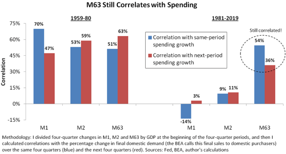
Moreover, since the B-Team understood money and banking better than everyone thought, M63 should be more reliable than M1 or M2. Its correlations should persist.
So do they?

Yes, M63 retained its correlations with spending. M1 and M2 did not.
So four decades after their 1980s pinnacle, the old-style monetarists, the data suggest, came tantalizingly close to achieving their goals. They weren’t completely wrong, they were just a little wide of the mark. Had they used M63 instead of the 1980s aggregates, the US money-supply obsession might have persisted.
Oh the Irony!
Now for the ironic part. In their seminal work, Monetary History of the United States, 1867–1960, Friedman and Schwartz based their thinking on the historical period spelled out in the title. But the M1 and M2 metrics didn’t exist until the end of that era.
So how did they measure the money supply when researching their book? They added up all the bank deposits and currency in circulation and called it all money. They used M63. And published their findings in 1963. Hence M63.
So M63’s obscurity is odd for three reasons:
- It captures the real-world Description B power of money.
- Its empirical record is better than M1’s or M2’s.
- It’s the “mother” aggregate — the metric that hooked economists on money supply in the first place.
So monetarists used M63 to develop their core ideas, but foisted the less powerful, single-digit M1, M2, etc., onto the public. That well-intentioned bait and switch facilitated the monetarists’ fall from influence.
What’s in It for You?
From a practical standpoint, by implication, M63 should help with forecasting. In fact, two data points suggest that M63 is something more than another metric worth tracking.
First, indicators drawn from the asset side of bank balance sheets, such as new bank credit, yield better results than those from the liability side, such as M63. The differences aren’t large, especially as new bank credit and M63 are highly correlated, but they are meaningful.
Second, M63 rejuvenates the equation of exchange that connects changes in GDP to those in either the money supply or the velocity of money. The equation isn’t helpful if the money measure — M1 or M2, for example — no longer correlates with spending. But M63 brings it back to life. By studying the velocity of M63 and its determinants, we can develop an outlook that’s more effective than relying on money (or bank credit) alone.
M63 is only a first look at Description B’s practical value. We can do even better by augmenting the long-forgotten M with other hidden ideas in macro.
For more from Daniel Nevins, CFA, don’t miss Economics for Independent Thinkers or its review in Enterprising Investor.
If you liked this post, don’t forget to subscribe to the Enterprising Investor.
All posts are the opinion of the author. As such, they should not be construed as investment advice, nor do the opinions expressed necessarily reflect the views of CFA Institute or the author’s employer.
Image credit: ©Getty Images/bernie_photo
[ad_2]
Image and article originally from blogs.cfainstitute.org. Read the original article here.


